What is Searching? Types of Searching

What is Searching? Types of Searching


  • Searching is the process of finding a given value position in a list of values.
  • It decides whether a search key is present in the data or not.
  • It is the algorithmic process of finding a particular item in a collection of items.
  • It can be done on internal data structure or on external data structure.
  • Searching Algorithms are designed to check for an element or retrieve an element from any data structure where it is stored.

Algorithms are generally classified into two categories:

  • Sequential Search: 

  • In this, the list or array is traversed sequentially and every element is checked. 

  • For example: Linear Search, Sentinel Linear Search

  • Interval Search: 

  • These algorithms are specifically designed for searching in sorted data-structures. 

  • These type of searching algorithms are much more efficient than Linear Search.

  • They repeatedly target the center of the search structure and divide the search space in half. 

  • For Example: Binary Search, Fibonacci Search

Sequential Search (Linear Search)

  • Sequential search is also called as Linear Search.
  • Sequential search starts at the beginning of the list and checks every element of the list.
  • It is a basic and simple search algorithm.
Sequential search compares the element with all the other elements given in the list. If the element is matched, it returns the value index, else it returns -1.

Complexity with example:

  34 56   21           09       76 1     98           50


Suppose,  key=34, we search it in array (where it is present or not in array)

Yes, It is present at arr[0] location that means we found it at 1st position,


We compare arr[i]==key and it takes O(1) time. This is the best time complexity of Linear search


Now we search key= 98, Again we compare arr[i]== key, it is located at 6th                        location, That means we get O(n) time complexity in average and worst case.


Pseudo Code: Linear Search


value=[2,5,6,9,1]

target= 9


function searchValue(value, target)

{

      for (var i = 0; i < value.length; i++)

      {

             if (value[i] == target)

             {

                     return i;

             }

      }

      return -1;

}


Binary Search

  • The binary search algorithm can be used with only a sorted list of elements.
  • Binary search follows divide and conquer approach in which, the list is divided into two halves.


Algorithm:

  1. This search process starts comparing the search element with the middle element in the list

  2. If both are matched, then the result is "element found".

  3. Otherwise, we check whether the search element is smaller or larger than the middle element in the list.

  4. If the search element is smaller, then we repeat the same process for the left sublist of the middle element.

  5. If the search element is larger, then we repeat the same process for the right sublist of the middle element. 

  6. if that element doesn't match with the search element, then the result is "Element not found in the list".

Example: 

1.The array in which searching is to be performed is:

Let, x= 4 element to be searched.


2. Set two pointers low and high at the lowest and the highest positions respectively.  Ie.,  low= 0 and high =6


3. Find the element  mid of the array ie. ([low+high])/2 =3 ie mid at 3rd location
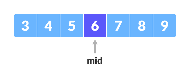

4. If x == arr[mid], then return mid. Else, compare the element to be searched with mid.

Ie. 4==6 


5.  If x>arr[mid]  compare x with middle element of  the elements of the right side of mid. Ie 4>6….? 

This is done by setting low to low= mid+1


6. Else, compare x with the middle of the elements on the left side of mid. 

7. Repeat steps 3 to 6 until low meets high
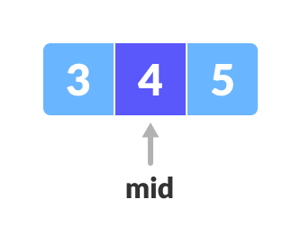
8. x=4 is found 

Pseudo Code:

This can be implemented in two ways which are discussed below.

  1. Iterative Method

  2. Recursive Method


  • Iterative Method

do until the pointers low and high meet each other.

mid = (low + high)/2

if (x == arr[mid])

    return mid

else if (x > A[mid]) // x is on the right side

    low = mid + 1

else                     // x is on the left side

   high = mid - 1


  • Recursive Method

The recursive method follows the divide and conquer approach.


binarySearch(arr, x, low, high)

  if low > high

      return False 

  else

      mid = (low + high) / 2 

      if x == arr[mid]

           return mid

      else if x < data[mid]        // x is on the right side

           return binarySearch(arr, x, mid + 1, high)

      else                       // x is on the right side

          return binarySearch(arr, x, low, mid - 1)


This is done by setting high to high= mid-1.   ie.  high = 3-1=2


  • Time Complexity:


  • Linear search time complexity is O(n).


  • Where Binary search has O(logn).


Fibonacci Search


 Similarities with Binary Search:

  1. Works for sorted arrays

  2. A Divide and Conquer Algorithm.

  3. Has Log n time complexity.

Differences with Binary Search:

  1. Fibonacci Search divides given array in unequal parts

  2. Binary Search uses division operator to divide range. Fibonacci Search doesn’t use /, but uses + and -. The division operator may be costly on some CPUs.

  3. Fibonacci Search examines relatively closer elements in subsequent steps. So when input array is big that cannot fit in CPU cache or even in RAM, Fibonacci Search can be useful.

This is based on Fibonacci series :


  • F(n+1)=F(n)+F(n-1)

  • where F(i) is the ith number of the Fibonacci series where F(0) and F(1) are defined as 0 and 1 respectively.

The first few Fibonacci numbers are:

0,1,1,2,3,5,8,13....

F(0) = 0

F(1) = 1

F(2) = F(1) + F(0) = 1 + 0 = 1

F(3) = F(2) + F(1) = 1 + 1 = 2

F(4) = F(3) + F(2) = 1 + 2 = 3 and so continues the series


Algorithm:  Let the length of given array be n [0...n-1] and the element to be searched be x.

  1. Find the smallest Fibonacci number greater than or equal to n. Let this number be fb(M) [m’th Fibonacci number]. Let the two Fibonacci numbers preceding it be fb(M-1) [(m-1)’th Fibonacci number] and fb(M-2) [(m-2)’th Fibonacci number].

  2. While the array has elements to be checked:

-> Compare x with the last element of the range covered by fb(M-2)

-> If x matches, return index value

-> Else if x is less than the element, move the third Fibonacci variable two Fibonacci down, indicating removal of approximately two-third of the unsearched array.

-> Else x is greater than the element, move the third Fibonacci variable one Fibonacci down. Reset offset to index. Together this results into removal of approximately front one-third of the unsearched array.


  1. Since there might be a single element remaining for comparison, check if fbM1 is '1'. If Yes, compare x with that remaining element. If match, return index value.


Example:  


Let the length of given array be n [0...n-1] and the element to be searched be x. 

    0              1                2                 3               4 //index

   2 3       5             7 8 // value


x=7      int arr[10];

N = sizeof(arr)/sizeof(arr[0])= 5


// Initialize fibonacci numbers

fibonacci(int arr[], int x, int n)

fbM2 = 0 // (m-2)'th Fibonacci number

fbM1 = 1; // (m-1)'th Fibonacci number

fbM = fbM2 + fbM1; // m'th Fibonacci

    // Marks the eliminated range from front

offset = -1;


// fbM is going to store the smallest Fibonacci

    number greater than or equal to n

while (fbM < n)

    {

        fbM2 = fbM1;

        fbM1 = fbM;

        fbM  = fbM2 + fbM1;

}


// fbM is going to store the smallest Fibonacci

    number greater than or equal to n

while (fbM < n)

    {

        fbM2 = fbM1;

        fbM1 = fbM;

        fbM  = fbM2 + fbM1;

}


// fbm=0+1=1;


while (2 < 5)

{

        fbM2 =1 ;

        fbM1 = 2;

        fbM  = 3;

}

while (3 < 5)

{

        fbM2 =2 ;

        fbM1 = 3;

        fbM  = 5;

}


//while there are elements to be inspected. Note that we compare arr[fibM2] with x. 

When fbM becomes 1,  fbM2 becomes 0 


while (fbM > 1)   // 5>1

    {

 int i = min(offset+fbM2, n-1);  // min(-1+2,4) 

i=1


int min(int x, int y)

{

    return (x<=y)? x : y;


if (arr[i] < x)  // 3<7

    {

        fbM  = fbM1;     fbM=3

        fbM1 = fbM2;   fbM1=2

        fbM2 = fbM - fbM1;   fbM2= 1

        offset = i;        offset=1

    }


else if (arr[i] > x)

    {

        fbM  = fbM2;

        fbM1 = fbM1 - fbM2;

        fbM2 = fbM - fbM1;

    }

else return i;

//element found. return index

} // close while loop

if (arr[i] < x)  // 3<7

    {

        fbM  = fbM1;     fbM=3

        fbM1 = fbM2;   fbM1=2

        fbM2 = fbM - fbM1;   fbM2= 1

        offset = i;        offset=1

    }


while (fbM > 1)   // 3>1

    {

 int i = min(offset+fbM2, n-1);  // min(1+2,4) 

i=3


if (arr[i] < x)  // 7<7

    {

        fbM  = fbM1;   

        fbM1 = fbM2;  

        fbM2 = fbM - fbM1;   

        offset = i;        

    }

else if (arr[i] > x)   // 7>7

    {

        fbM  = fbM2;

        fbM1 = fbM1 - fbM2;

        fbM2 = fbM - fbM1;

    }

else return i;

//element found. return index

} // close while loop

/* comparing the last element with x */


  if(fbM1 && arr[offset+1]==x)

    return offset+1;


 /*element not found. return -1 */

    return -1;


Complexity:
  • Worst case time complexity: O(logn)
  • Average case time complexity: O(logn)
  • Best case time complexity: O(n)
  • Space complexity: O(1)

Program:
#include<iostream> #include<conio.h> /* Find min of given number */ int min(int x, int y) { return (x<=y)? x : y; } /* Returns index of x if present, else returns -1 */ int fibonaccianSearch(int arr[], int x, int n) { /* Initialize fibonacci numbers */ int fbM2 = 0; // (m-2)'th Fibonacci number int fbM1 = 1; // (m-1)'th Fibonacci number int fbM = fbM2 + fbM1; // m'th Fibonacci // Marks the eliminated range from front int offset = -1; /* fbM is going to store the smallest Fibonacci number greater than or equal to n */ while (fbM < n) { fbM2 = fbM1; fbM1 = fbM; fbM = fbM2 + fbM1; } /* while there are elements to be inspected. Note that we compare arr[fibM2] with x. When fbM becomes 1, fbM2 becomes 0 */ while (fbM > 1) { // Check if fbM2 is a valid location int i = min(offset+fbM2, n-1); /* If x is greater than the value at index fbM2, cut the subarray array from offset to i */ if (arr[i] < x) { fbM = fbM1; fbM1 = fbM2; fbM2 = fbM - fbM1; offset = i; } /* If x is greater than the value at index fbMm2, cut the subarray after i+1 */ else if (arr[i] > x) { fbM = fbM2; fbM1 = fbM1 - fbM2; fbM2 = fbM - fbM1; } /* element found. return index */ else return i; } /* comparing the last element with x */ if(fbM1 && arr[offset+1]==x) return offset+1; /*element not found. return -1 */ return -1; } /* main function */ int main(void) { clrscr(); int l; cout<<"\nEnter the number of elements in array which should be less than 10"; cin>>l; int arr[10]; cout<<"Enter elements in array"; for(int i=0;i<l;i++) { cin>>arr[i]; } int n = sizeof(arr)/sizeof(arr[0]); int x; cout<<"\nEnter element to be searched :" ; cin>>x; cout<<"Found at index:"<<fib1onaccianSearch(arr, x, n); getch(); return 0; }

netaji gandi Thursday, April 28, 2022
Data Structure, ADT and Type of data structure


Abstract Data Type (ADT):
  • A data type can be considered abstract when it is defined interms of operations on it with its implementation is hidden
Definition:
  • A set of data types & associated operations that are precisely specified, independent of any particular implementation.

Example: Common examples are built in primitive types, i.e int ,char, float, etc.


Data Structure :
  • A data structure is a specialized format for organizing, processing, retrieving and storing data.
  • A data structure is a particular way of organizing data in a computer so that it can be used effectively.
Properties of Data Structure:
  1. Every data structure is used to organise large amount of data.
  2. Every data structure follows particular principle
  3. Operations in data structure should not violate its basic principles
Types of Data Structures:
  • There are two types of data structures such as primitive and non-primitive.
  • Primitive data structures are all inbuilt data types. Where non primitive data structures are generated by using primitive data types.


Linear Data Structure:
  • If a data structure is organising data sequentially then that data structure is linear data structure
  • A Linear data structure have data elements arranged in sequential manner and each member element is connected to its previous and next element. 
  • This connection helps to traverse a linear data structure in a single level and in single run.
Example:

  • Array: Fixed size
  • Linked list: Variable size

  • Stack: LIFO
  • Queue: FIFO

Non Linear Data Structure:
  • If a data structure organises data in random order, then that data structure is called non linear data structure
  • A non-linear data structure has no set sequence of connecting all its elements and each element can have multiple paths to connect to other elements.
Example: 

  • Tree
  • Graph
Fig : Non linear data structure

Static Data Structure:
  • It is an organisation or collection of data in memory that is fixed in size
  • This result in maximum size needing to be known in advance, as memory cannot be reallocated later 
Example:   All inbuilt data type, newspaper


Dynamic Data Structure:
  • We can change its size.
  • Where in with the later, the structure size can  dynamically grow or shrink as need.
  • They are flexible to consume additional memory if needed or free up memory when possible for improved efficiency.
Example: Linked list, web pages

Persistent Data Structure:


It is one where multiple versions are simultaneously accessible where after an update both old and new version can be used.

This data structure always preserves previous version of itself on modification.Such data Data structure is fully persistent if every version can be both accessed and modified.
 Example: tuple, string

Ephemeral Data Structure:

An EDS is one for which only one version is available at a time, after update the structure as it existed before updation is lost.
  • In imperative languages, most data structures are ephemeral
  • Much of data stored on computers like like data stored on RAM & caches is temporary & thus is referred  as ephemeral.
  • This temporary, transient files are deleted as often as every few hours.
  • Such data structure are mutable
Example:  list, set and dictionary

Performance Analysis:

  • There are multiple algorithms to solve a problem. When we have more than one algorithm, we need to select one.
  • Performance of an algorithm means predicting the resources which are required to an algorithm to perform its task.

  • Performance analysis helps us to select the best algorithm to solve a problem.

  • Performance analysis of an algorithm is the process of calculating space and time required by that algorithm.

Complexity:
  • Complexity of an algorithm is a function f(n) which measures time and space used by an algorithm in terms of input size ‘n’.
  • Algorithm complexity is commonly represented with the O(f) notation.
Complexity has two types:
     1. Time complexity
     2. Space complexity

Space Complexity:

Total amount of computer memory required by an algorithm to complete its execution is called as space complexity of that algorithm.

When we design an algorithm to solve a problem, it needs some computer memory to complete its execution. For any algorithm, memory is required for the following purposes:
  1. To store program instructions.
  2. To store constant values.
  3. To store variable values.
  4. And for few other things like function calls, jumping statements etc,.
Generally, when a program is under execution it uses the computer memory for THREE reasons. They are as follows....

Instruction Space: It is the amount of memory used to store compiled version of instructions.

Environmental Stack: It is the amount of memory used to store information of partially executed functions at the time of function call.

Data Space: It is the amount of memory used to store all the variables and constants.


Time Complexity:

The time complexity of an algorithm is the total amount of time required by an algorithm to complete its execution.

Generally, the running time of an algorithm depends upon the following:

1. Whether it is running on Single processor machine or Multi processor Machine.

2. Whether it is a 32 bit machine or 64 bit machine.

3. Read and Write speed of the machine.

4. The amount of time required by an algorithm to perform Arithmetic operations, logical operations, return value, assignment operations and input data.

Constant Time Complexity:

If any program requires a fixed amount of time for all input values then its time complexity is said to be Constant Time Complexity.

Linear Time Complexity:

If the amount of time required by an algorithm is increased with the increase of input value then that time complexity is said to be Linear Time Complexity.


Asymptotic Notation:
  • Asymptotic notation of an algorithm is a mathematical representation of its complexity.
  • Asymptotic Notations are the expressions that are used to represent the complexity of an algorithm.
Types of Asymptotic Notation:

  • Big - Oh (O)
  • Big - Omega (Ω)
  • Big - Theta (Θ)

Big - Oh Notation (O):

  • Big - Oh notation is used to define the upper bound of an algorithm in terms of Time Complexity.
  • That means Big - Oh notation always indicates the maximum time required by an algorithm for all input values.
  • That means Big - Oh notation describes the worst case of an algorithm time complexity.

Definition:
Consider function f(n) as time complexity of an algorithm and g(n) is the most significant term. If f(n) <= C g(n) for all n >= n0, C > 0 and n0 >= 1. Then we can represent f(n) as O(g(n))
f(n) = O(g(n))

Consider the following graph drawn for the values of f(n) and C g(n) for input (n) value on X-Axis and time required is on Y-Axis


In above graph after a particular input value n0, always C g(n) is greater than f(n) which indicates the algorithm's upper bound.

Example:
We are creating array with size= 9
int a[9];

Case 1:
Suppose we want to search number 9 in the array: 9 is located at 8th index. It takes O(n) time for traversing this number.  

Case 2:
Suppose we want to search 55 number in the array.

Example:
Consider the following f(n) and g(n)...
f(n) = 3n + 2
g(n) = n

If we want to represent f(n) as O(g(n)) then it must satisfy f(n) <= C g(n) for all values of C > 0 and n0>= 1
    f(n) <= C g(n)
    3n + 2 <= C n
    f(n)=3*2+2=8
    cn=4*2=8
    8<=8

Above condition is always TRUE for all values of C = 4 and n >= 2.
By using Big - Oh notation we can represent the time complexity as follows....
3n + 2 = O(n)


Big - Omege Notation (Ω):
  • Big - Omega notation is used to define the lower bound of an algorithm in terms of Time Complexity.
  • That means Big-Omega notation always indicates the minimum time required by an algorithm for all input values. 
  • That means Big-Omega notation describes the best case of an algorithm time complexity.

Definition:
Consider function f(n) as time complexity of an algorithm and g(n) is the most significant term. If f(n) >= C g(n) for all n >= n0, C > 0 and n0 >= 1. Then we can represent f(n) as Ω(g(n)).
f(n) = Ω(g(n))

Example:
We are creating array with size= 9
int a[9];

Case 1:
Suppose we want to search number 12 in the array: 12 is located at 0th index. It takes O(1) time for traversing this number.  

Case 2:
Suppose we want to search 45 number in the array.

Consider the following graph drawn for the values of f(n) and C g(n) for input (n) value on X-Axis and time required is on Y-Axis


In above graph after a particular input value n0, always C g(n) is less than f(n) which indicates the algorithm's lower bound.

Example:

Consider the following f(n) and g(n)...
f(n) = 3n + 2
g(n) = n

If we want to represent f(n) as Ω(g(n)) then it must satisfy f(n) >= C g(n) for all values of C > 0 and n0>= 1
f(n) >= C g(n)
⇒3n + 2 >= C n

Above condition is always TRUE for all values of C = 1 and n >= 1.
By using Big - Omega notation we can represent the time complexity as follows....
3n + 2 = Ω(n)


Big - Theta Notation (Θ):
  • Big - Theta notation is used to define the average bound of an algorithm in terms of Time Complexity.
  • That means Big - Theta notation always indicates the average time required by an algorithm for all input values. 
  • That means Big - Theta notation describes the average case of an algorithm time complexity.

Definition:
Consider function f(n) as time complexity of an algorithm and g(n) is the most significant term. If C1 g(n) <= f(n) <= C2 g(n) for all n >= n0, C1 > 0, C2 > 0 and n0 >= 1. Then we can represent f(n) as Θ(g(n)).
f(n) = Θ(g(n))

Example:
We are creating array with size= 9
int a[9];

Case 1:
Suppose we want to search number 54 in the array: 54 is located at 3rd index. O(3) is the  Time complexity for searching 54.  

Case 2:
Suppose we want to search 67 number in the array.

Consider the following graph drawn for the values of f(n) and C g(n) for input (n) value on X-Axis and time required is on Y-Axis.

In above graph after a particular input value n0, always C1 g(n) is less than f(n) and C2 g(n) is greater
than f(n) which indicates the algorithm's average bound.

Example:

Consider the following f(n) and g(n)...
f(n) = 3n + 2
g(n) = n

If we want to represent f(n) as Θ(g(n)) then it must satisfy C1 g(n) <= f(n) <= C2 g(n) for all values of C1 > 0, C2 > 0 and n0>= 1
C1 g(n) <= f(n) <= C2 g(n)
⇒C1 n <= 3n + 2 <= C2 n
C1n=2
f(n)=3*2+2=8    c2(f(n))= 4*2=8

Above condition is always TRUE for all values of C1 = 1, C2 = 4 and n >= 2.
By using Big - Theta notation we can represent the time complexity as follows....
3n + 2 = Θ(n).


Analysis of Programming Constructs:   


Algorithmic Strategies:

  • General approaches to the construction of efficient solution to problems
  • Some methods provide templates suited to solving broad range of diverse problem
  • Although more than 1 technique may be applicable to a specific problem, it is often the case that algorithm constructed by certain approach is clearly superior to equivalent solution built using alternative techniques

There are different types of Algorithmic Strategies:
1. Divide and Conquer
2. Greedy method
3. Backtracking
4. Branch and bound
5. Dynamic programming

Divide and Conquer:

Divide-and-conquer, breaks a problem into subproblems that are similar to the original problem, recursively solves the subproblems, and finally combines the solutions to the subproblems to solve the original problem. 

Divide: the original problem into a set of subproblems.
Conquer: Solve every subproblem individually, recursively.
Combine: Put together the solutions of the subproblems to get the solution to the whole problem.

Divide and Conquer

Examples:
The specific computer algorithms are based on the Divide & Conquer approach:
  • Binary Search
  • Merge sort
  • Maximum and Minimum Problem
  • Quick sort
  • Tower of Hanoi
Greedy method:
  • This makes the choice that seems to be the best at that moment. 
  • This means that it makes a locally-optimal choice in the hope that this choice will lead to a globally-optimal solution.
  • The Greedy algorithm has only one shot to compute the optimal solution so that it never goes back and reverses the decision.
Example:
  • Minimum Spanning Tree
  • Fractional Knapsack Problem
  • Graph vertex cover
  • Huffman tree
  • Job Sequencing problem

netaji gandi Friday, April 22, 2022
Introduction to Algorithm and Data Structures

 Difference Between Data, Information and Knowledge


Data: 

    We always use word data. Data is collection of symbol,mnemonics, digit, elementary description of things, events, activities and transactions that are recorded, classified and stored but are not organized to convey any specific meaning.

Information:

    When we perform some operations or process on data Data it converts into information. Information have meaning and value to the recipient.

Knowledge:

    Data and/or information organized and processed to convey understanding, experience, accumulated learning and expertise as they apply to a current problem or activity.


Problem Solving:

To solve a given problem by using a computer, we need to write a program for it .

A program consists of two components as follows:
                        

Algorithm:

It can be defined as a step by step procedure for solving a particular problem

Characteristic of Algorithm:

1. Unambiguous : Algorithm should be clear. Each of its steps and their input output should be clear and must lead to only one meaning.

2. Input : An algorithm should have 0 or more well defined input

3. Output: An algorithm should have 1 or more well defined output. 
 
4. Finiteness : Algorithm must terminate after finite no. of steps

5. Feasibility : Should be feasible with available resources.

6. Independent: An algorithm should have step by step directions, which should be independent of any programming code  


 Algorithm Design Tools:


1. Pseudo Code: 
  • Consists of natural language like statements that enables the programmer to plan without worrying about syntax.
  • Statements describe actions
  • Focuses on logic of the algorithm/ program
  • It neither an algorithm nor a program
Example: Program for Addition of two nos.
                  
                    Add()
                    {
                    a=input number
                    b=input number
                    c=addition of a+b
                    print(c)
                    }

2. Flowchart:  
  • A flowchart is a graphical or symbolical representation of an algorithm
  • It is a diagram that describes a process or operation
There are large number of symbols used for drawing flowchart. Some of them are as follows:

1. Oval: This shape is also called as 'Terminator Symbol'. 
                                
Terminator


This oval shape symbol represents the start or end of process. We always write 'start', 'end' ,'begin' or 'stop' inside it.

2. Rectangle:  This is also referred as 'action symbol'.


This rectangle shape symbol represents 'action', 'operation', 'function' or 'process'. This is most widely used symbol for drawing flowchart.

3. Parallelogram: This is also referred as 'data symbol'.

This symbol represents input and output (Information entering and leaving) of the system.

4. Diamond: This symbol represents 'Decision'. It is used in a process flow to ask a question and the answer is terms of arrows coming out diamond. It takes decision as 'yes/no' or 'true/false'.


5. Circle: This symbol connects separate elements across one page. It represents continuous flow with matching symbol.

6. Arrow:  This represents 'connection' and 'relationship' from one symbol to another using arrow. 

Example:
                 Find out whether number is even or odd 
Flowchart:


netaji gandi

Java Programming Lab

☕ Java Programming Lab Select a laboratory session to view programs and documentation Week 01 ...